6. Pages¶

Every network graph, table, list, line chart available in TIM is displayed in a Page.

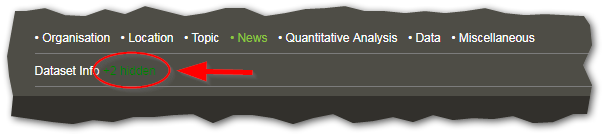
Pages are organised into categories, for better navigation, as can be seen in the following figure. To select a page, first select a category and then one of the available pages below. What you have selected is highlighted in green.

catPages

There is a special type of pages called space pages, that show visualisations not for a single dataset, but on all the datasets available in the space.

There are pages that are pre-configured and that the User has no control over; these are called default pages. There are other pages that are configurable by the User, called custom pages, that can be created initially from a default page and then modified as seen fit; they can also be entirely created from scratch.

Custom pages can be created also for space pages; these are–naturally–called Custom space pages.

The categories available are the following:

Organisation: Network graph visualizations relating to the organisations/entities that are publishing, patenting or are beneficiaries of EU projects.
Location: Network graph visualisations relating to the location of the organisations detected in the documents. Different levels of granularity are available, from countries to regions and cities. There is also a geographic projection on a map.
Topic: Visualisations that relate to the topic of the documents in the dataset.
News: Direct access to the latest news on the specific emerging technologies and news trends.
Quantitative analysis: Trends and indicators calculated on the dataset. Filters apply to the data.

Sometimes, some default pages are hidden. In order to make them appear again, click on the hidden link, as seen below, and then out of the list, select which page you want to unhide. After closing this window, the pages of the category have cogwheels next to them. Clicking on the cogwheel gives you the option to hide a default page, or delete a custom page.

hidden

6.1. Default Pages¶

The set of pages available to basic, advanced and lab users follows. More information on what the pages show is given in Page Categories

Category	Page	Visualisation	Description
Space Page	Datasetgram	Network graph	The nodes are the datasets in the space and their size is the number of documents. The edges represent the documents in common.
	News Trends	Charts	News trends for all datasets associated to a news category. Only available if the news category have been previously created.
	Dataset Matrix (L)	Matrix	All datasets displayed in a matrix. The intersection of two datasets represents the number of documents in common. A list of all the datasets is also available.
Organisation	Dataset Info	Text	Information about the dataset (name, search string, creation and modification date, distribution in types of documents, trend in time and more).
Organisation	Organisations	Network graph	The nodes are the Top 100 Organisations (Processed names 1). The edges represent Co-patenting and/or Co-publishing and/or Co-participation in an EU research project(s).
Location	Dataset Info	Text	See above
	Cities	Network graph	The nodes are the Top 100 cities where the Organisations (processed) are located. The edges represent Co-patenting and/or Co-publishing and/or Co-participation in an EU research project(s) between the organisations in those cities.
	Countries	Network graph	The nodes are the countries where the Organisations (processed 1) are located. The edges represent Co-patenting and/or Co-publishing and/or Co-participation in an EU research project(s) between the organisations in those countries.
	EU/World	Network graph	The nodes are the EU countries (all in one node) or rest of the world countries where the Organisations (processed) are located. The edges represent Co-patenting and/or Co-publishing and/or Co-participation in an EU research project(s) between the organisations in those countries.
	EU Countries	Network graph	The nodes are the EU countries where the Organisations (processed 1) are located. The edges represent Co-patenting and/or Co-publishing and/or Co-participation in an EU research project(s) between the organisations in the EU countries.
	NUTS2	Network graph	The nodes are the Nuts2 regions where the Organisations (processed) are located. The edges represent Co-patenting and/or Co-publishing and/or Co-participation in an EU research project(s) between the organisations in those regions of the EU.
	NUTS3	Network graph	The nodes are the Nuts3 regions where the Organisations (processed) are located. The edges represent Co-patenting and/or Co-publishing and/or Co-participation in an EU research project(s) between the organisations in those regions of the EU.
	Map	Map	Location of the Organisations (processed) in a geographical map based on the location of the city. The circles or pointers on the map indicate the number of documents in the area that appears when hovering.
	EU/World Map	Map	Location of the Organisations (processed) in a geographical map with all the EU as one location. The circles or pointers on the map indicate the number of documents in the area that appears when hovering. Documents from organisations in the EU are forced to appear as one unique location in Brussels.
	Heatmap Country (adv)	Heatmap	Location of the Organisations (processed) in a heatmap. The gradation of colours in the countries indicates the number of documents in the specific country.
	Heatmap EUCountry (adv)	Heatmap	Location of the Organisations (processed) in a heatmap. The gradation of colours in the countries indicates the number of documents in the in the specific country. Documents from organisations in the EU are forced to appear as one mega-region covering the European countries.
	Inventor Country (adv)	Network graph	The nodes are the countries where the Inventors of the patents reside. The edges represent Co-patenting between the inventors residing in those countries. (Only available for patents)
	Heatmap Nuts2 (L)	Heatmap	Location of the Organisations (processed) in a heatmap. The gradation of colours in the Nuts2 regions indicates the number of documents in the specfic region.
	Heatmap Nuts3 (L)	Heatmap	Location of the Organisations (processed) in a heatmap. The gradation of colours in the Nuts3 regions indicates the number of documents in the specfic region.
	World graph (L)	Map	Organisations (processed) location in a geographical map with edges representing collaboration.
Topic	Dataset Info	Text	See above
	Journal categories (S)	Network graph	The nodes are the scientific categories to which the journals where the scientific publications are published belong. The edges represent the co-ocurrence of two categories in the same document, i.e. documents published in journals that are assigned to both categories. (Only available for scientific publications)
	Detailed patent classification	Network graph	The nodes are the CPC classification symbol (full version) to which the patent is attributed. The edges represent the co-ocurrence of two CPC classes in the same patent, i.e. inventions that belong to both subjects. (Only available for patents)
	Author keywords (S)	Network graph	The nodes are the Author keywords (cleaned 2) attributed by the authors to their publications. The edges represent the co-ocurrence of two author keywords in the same publication. (Only available for scientific publications)
	Automatic keywords	Network graph	The nodes are the Automatic keywords 2 generated by language processing algorithms for all types of documents. The edges represent the co-ocurrence of two automatic keywords in the same document.
	Scholar keywords (SS)	Network graph	The nodes are keywords generated by AI algorithms used by Semantic Scholar. The edges represent the co-ocurrence of two Scholar keywords in the same document.
	Relevant Keywords	Text	Most relevant keywords 2 in the dataset and their relevance. These keywords are generated by language processing algorithms to represent the dataset as a whole.
	Patent classification (adv)	Network graph	The nodes are the CPC subclasses (5 digits + name) to which the patent is attributed. The edges represent the co-ocurrence of two CPC classes in the same patent, i.e. inventions that belong to both subjects. (Only available for patents)
	Classification(5)gram (adv)	Network graph	The nodes are the CPC subclasses (5 digits) to which the patent is attributed. The edges represent the co-ocurrence of two CPC classes in the same patent, i.e. inventions that belong to both subjects. (Only available for patents)
	Documentgram (adv)	Network graph	The nodes are the documents in the dataset. The edges represent the semantic similarity between two documents.
	Author Keywords (Raw) (adv)	Network graph	The nodes are the raw version of the Author keywords attributed by the authors to their publications. The edges represent the co-ocurrence of two author keywords in the same publication. (Only available for scientific publications)
	Clusters (adv)	Network graph	The nodes are clusters of documents based on their semantic similarity. The name of the cluster is the most relevant keyword of the cluster of documents. The edges represent the semantic similarity between clusters of documents.
	Author Keywords List (Raw) (L)	Text	List of Author keywords (raw) attributed by the authors to their publications. (Only available for scientific publications)
	Automatic Keyword List (L)	Text	List of the Automatic keywords attributed by TIM to all types of documents.
Quantitative Analysis	Dataset Info	Text	See above
	Type of documents (adv)	Chart	Chart and table of the distribution of each type of document per year in the dataset.
	Time series (adv)	Chart	Chart and table of the evolution in time of the number of documents per organisation.
News	Dataset Info	Text	See above
	News (adv)	Text	Latest news for the EMM category assigned to the dataset. (Only available if a news category has been previously created.)
	News Trends (adv)	Chart	Evolution in time of the number of news items retrieved (Only available if a news category has been previously created.)
Miscellaneous	Dataset Info	Text	See above
	Years	Network graph	The nodes are the publication year of the publication, priority year of the patent or starting year of the EU project. There are no edges in the graph, as a document cannot have two differente years. Use this graph for filtering purpouses.
	Type of documents	Network graph	The nodes are the types of documents in the dataset. There are no edges in the graph, as a document cannot be of two different types. Use this graph for filtering purposes.
	Data source	Network graph	The nodes are the Original database from where the documents come from. There are no edges in the graph, as a document cannot come from two different databases. Use this graph for filtering purposes.
	Documents	Text	List of documents in the dataset.
Data (adv)	Dataset Info	Text	See above
	Rss (adv)	Text	Dataset in RSS format.
	Json (adv)	Text	Dataset in Json format.
	Field Viewer (adv)	Text	All fields and values of the dataset displayed in a user friendly and filterable way.
	Transformation status (adv)	Text	System page that informs about the status of user defined and system transformations.
	Main fields (L)	Text	Main fields (title and descriptions) and values of the dataset displayed in a user friendly and filterable way.
Lab (L)	Dataset Info	Text	See above
	Collaborations (L)	Chord diagram	Chords diagram with organisations countries to analyse The edges represent the co-ocurrence of two specific values of the same or different field.
	MixedGram (L)	Network Graph	The nodes are the values of two different fields, countries and years.
	Pub Citations (L)	Directed Network Graph	The nodes are the publications in the dataset. The edges represent the citations from one publication to the other (Only available for scientific publications)
	Patent citations (L)	Directed Network Graph	The nodes are the patents in the dataset. The edges represent the citations from one patent to the other. (Only available for patents)

Pages with (SS) are only available where the Semantic Scholar database is available, for now TIM Open Access.
Pages with (S) are only available where the Scopus database is available (unavailable in TIM Open Access).

Pages with (adv) are only available to users who have the advanced role enabled.
Pages with (L) are only available to users who have the Lab role enabled.

Warning

Not all pages are available for all groups of documents. Also, not all pages are available by default to all user roles. The user role can be modified by the Users themselves. See User Roles in TIM for more information.

Note

As TIM is in continous development, some new pages may be added and/or some outdated ones may be removed without notice. The list below might not reflect accurately the currently available pages.

6.2. Custom Pages¶

The User can create a Custom Page to display data from the TIM database that don’t already have a page to visualise it, or to display new data, by either applying a custom transformation, or by applying an Indicator.

There are different types of Custom Pages, and the most important ones available are the gram and the Time Series Custom Page. The gram Custom Page is behind all the built-in network graph visualisations that are available in TIM and it can also be used to visualise the data in lists. The Quantitative Analysis>Time Series is a Time Series custom Page: it plots data in a simple X-Y graph with the time variable always in the X-axis.

There are also two places that the Custom Page can be created from, and this affects where and how it is available. There are Space-level Custom Pages and User-level Custom Pages.

Note

The user-defined custom pages are specific either to the Space or to the User. In the first case, they will be visible only in that Space and hence also for other users that might have viewing or editing rights on the space. If the custom page is defined at the User level, it will be visible on all Spaces of that User, but not for other Users that might be sharing the same space(s).

6.2.1. How to create a custom Page¶

The most straightforward way to create a custom page is to create one based on a pre-existing page. To do so, go to one of the available pages (e.g. Organisation>Organisations) and then click on the Edit icon on the top right of the page. Since this page is a built-in page, it is not actually editable; TIM, instead, will create a new custom page based on the built-in page, in the Space level. The new page is created on the same category as the built-in page, with a predefined but editable name. After you select it, you can click on the Edit button again and customize it further, using the dialog that will show up.

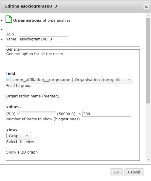
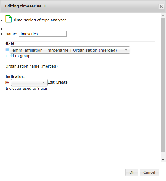
The picture on the left is the options available to the gram-type pages, and the picture on the right is the options available to the Time Series-type pages.

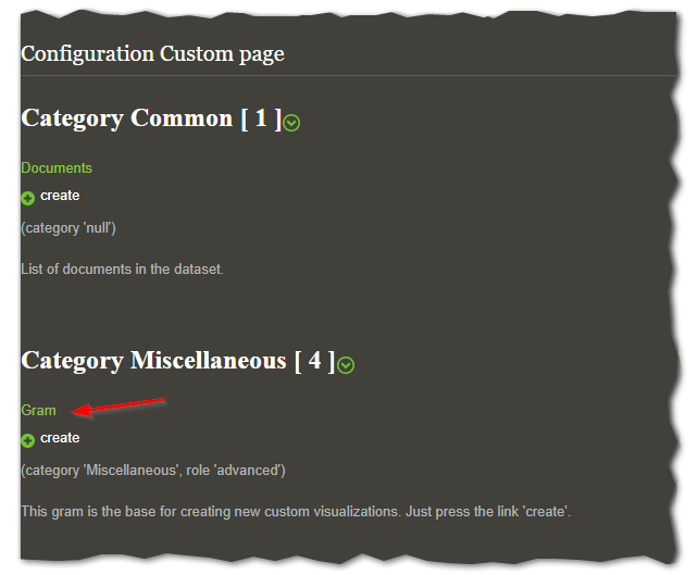
To create a User-level Custom Page, click on More on the top right-hand side of the screen, and then Settings>Pages and Visualisations>Custom Page.

To create a User-level Custom Space Page, click on More on the top right-hand side of the screen, and then Settings>Pages and Visualisations>Custom Space Page.

A list of Custom Page categories will show up, the most commonly used one is Miscellaneous>Gram.

CustomPageUser

The options available for Gram and Time Series follow.

6.2.1.1. Gram Options¶

6.2.1.1.1. Name¶

Here you select a name for the Custom Page.

6.2.1.1.2. Field¶

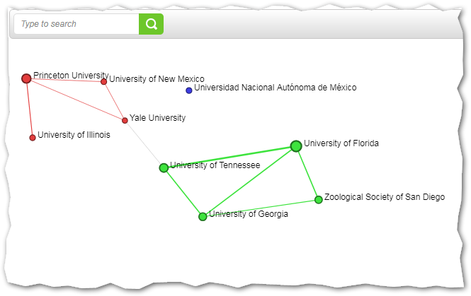
Here you select what the nodes on the graph represent. For example, the default organisations page shows emm_affiliation__mrgename [Organisation name (merged)] nodes. You can just type in the field you are looking for, or select it from the dropdown menu. The field names are followed by a short description. For a full list of fields available in TIM, see Fields in TIM.

6.2.1.1.3. Values¶

Here you can select how many items (= number of nodes) you want to see. The default organisations page shows the biggest 100 organisations for the selected dataset. If you want a more detailed graph, you can set this to the maximum (50,000), but loading and navigating the graph will be slower.

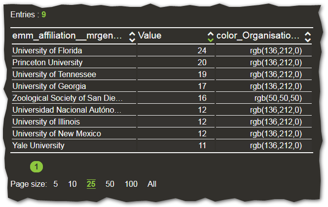
6.2.1.1.4. View¶

Here, there are two options for the advanced user: graph and list. Graph is the default view, a list shows the same information in a customiseable table format.

6.2.1.1.5. Indicators¶

The default behaviour of TIM is that the size of each node reflects the number of documents that belong to the node, and the same goes for the thickness of the edge between two nodes. This is calculated by an indicator that counts the number of documents that belong to the node. In this section, you have the possibility to select a different indicator for each node and/or edge. For more information on indicators, please see indicators.

Note

Indicators can be created and edited also from the Space Settings Page.

6.2.1.2. Time Series Options¶

6.2.1.2.1. Name¶

Here you select a name for the Custom Page.

6.2.1.2.2. Field¶

Here you select what the data points on the time series represent. For example, the default time-series page shows the number of documents per year for each organisation (emm_affiliation__mrgename) (The x-axis is always the year; it’s a time series after all!). For a full list of fields available in TIM, see Fields in TIM.

6.2.1.3. Indicator¶

The indicator that you select here determines what the number on the y-axis represents. The default is the Count indicator, which just counts the number of documents per node (here, per organisation). For more information on Indicators, please see here.

Warning

Please be aware that some indicators may be time-dependent (e.g. activeness). In this case, a visualisation as a times series might not yield meaningful results.

6.3. Space Pages¶

When first opening TIM, no specific dataset is selected. Another set of pages called Space pages is then displayed, presenting data that is relative to all the datasets as a whole.

timLandingPage1

To go back to the space pages when you are already in a specific dataset, simply click on the TIM logo on the top left to deselect any active dataset.

The default space page is the Datasetgram.

6.3.1. Datasetgram¶

The datasetgram is a network graph of all the datasets that have been created in the current space.

timLandingPage2

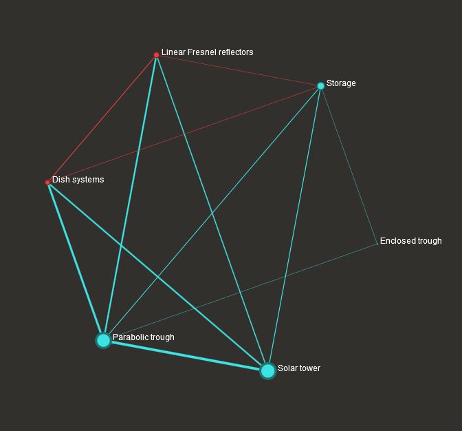
In this visualisation, each node is a dataset (a query that was made). The size of the nodes corresponds to the number of documents retrieved for each dataset. The edges between the nodes are documents in common in between the two datasets. The thicker the edge, more documents are in common. The colours show the communities of nodes, i.e. datasets that tend to have more data in common with each other than with the nodes of a different colour.

1(1,2,3): To learn more about the processing of affiliations, read Affiliation processing.
2(1,2,3): To learn more about the text processing for keywords, read Text Processing algorithms for keywords.